What the Swiss FX shock says about risk models
What the Swiss FX shock says about risk models
This page accompanies the VoxEU article What the Swiss FX shock says about risk models on January 18, 2015.
A daily updated franc risk is shown on my risk forecast page, and some additional analysis on the Swiss event is here.
Overview
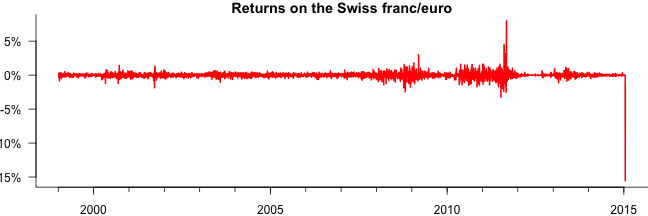
I downloaded the daily Swiss franc/euro exchange rate from the ECB, you can find the resulting CSV file here.
To start with, see the plot of the exchange rate
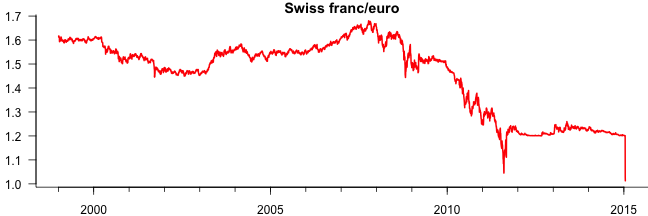
and the daily log returns $$y_t=\log\left(p_t/p_{t-1}\right)$$.
Data used in the estimation
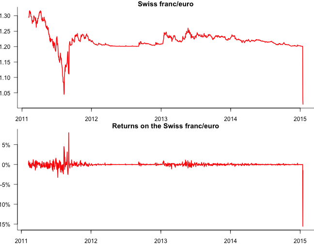
The estimation window is 1000 days and so consider the last 1010 days of the sample:
Results 1
The risk measures considered are historical simulation (HS), moving average normal (MA), exponentially weighted moving average normal (EWMA), normal GARCH, student-t GARCH and extreme value theory (EVT). The probability is 0.01, the estimation window is 1010 days and the risk measures are Value-at-Risk (VaR) and expected shortfall (ES). The risk is based on a portfolio of € 1,000.
The code to estimate comes from my risk library, which extends the code from financial risk forecasting.
so then on a euro 1000 portfolio
| day | fx | return | HS.VaR | HS.ES | MA.VaR | MA.ES | EWMA.VaR | EWMA.ES | GARCH.VaR | GARCH.ES | tGARCH.VaR | tGARCH.ES | EVT.VaR | EVT.ES |
|---|---|---|---|---|---|---|---|---|---|---|---|---|---|---|
| 6 Jan 2015 | 1.2014 | -0.02% | 14.04 | 20.33 | 11.48 | 13.15 | 1.93 | 2.21 | 2.18 | 2.50 | 3.30 | 4.55 | 13.90 | 24.41 |
| 7 Jan 2015 | 1.2011 | -0.02% | 14.04 | 20.33 | 11.48 | 13.15 | 1.89 | 2.17 | 2.09 | 2.40 | 3.16 | 4.36 | 13.90 | 24.41 |
| 8 Jan 2015 | 1.201 | -0.01% | 14.04 | 20.33 | 11.47 | 13.14 | 1.84 | 2.11 | 2.05 | 2.35 | 2.94 | 4.06 | 13.90 | 24.41 |
| 9 Jan 2015 | 1.201 | 0.00% | 14.04 | 20.33 | 11.45 | 13.11 | 1.79 | 2.05 | 1.84 | 2.11 | 2.78 | 3.83 | 13.90 | 24.41 |
| 12 Jan 2015 | 1.201 | 0.00% | 14.04 | 20.33 | 11.44 | 13.11 | 1.74 | 1.99 | 1.73 | 1.98 | 2.59 | 3.58 | 13.90 | 24.41 |
| 13 Jan 2015 | 1.201 | 0.00% | 14.04 | 20.33 | 11.44 | 13.11 | 1.69 | 1.93 | 1.62 | 1.86 | 2.43 | 3.35 | 13.90 | 24.41 |
| 14 Jan 2015 | 1.201 | 0.00% | 14.04 | 20.33 | 11.43 | 13.09 | 1.64 | 1.88 | 1.78 | 2.04 | 2.26 | 3.11 | 13.90 | 24.41 |
| 15 Jan 2015 | 1.028 | -15.55% | 14.04 | 20.33 | 11.42 | 13.09 | 1.59 | 1.82 | 1.71 | 1.96 | 2.10 | 2.89 | 13.90 | 24.41 |
| 16 Jan 2015 | 1.0128 | -1.49% | 14.40 | 34.48 | 16.16 | 18.51 | 11.34 | 12.99 | 13.59 | 15.57 | 1.96 | 2.71 | 15.65 | 31.18 |
| 19 Jan 2015 | 14.90 | 34.53 | 16.19 | 18.55 | 89.36 | 102.37 | 123.48 | 141.47 | 218.01 | 301.09 | 15.89 | 31.47 |
| MA | EWMA | GARCH | tGARCH | EVT | |
|---|---|---|---|---|---|
| probability | 1.5e-220 | 0.0e+00 | 0.0e+00 | 2.9e-10 | 3.7e-05 |
| frequency in years | 2.74e+217 | Inf | Inf | 1.39e+07 | 1.09e+02 |
Why the model forecasts are consistent with the data
Start with the last figure.
- HS VaR uses the 1% quantile, and that does not pick up on the main event, the ES will be much more affected by the event because it will get a 10% weight in the sum
- moving average VaR and ES are falling before the event because the volatilities trending down, and with the event getting a 0.1% weight, it should be picked up but not too much
- EWMA VaR and ES would be trending sharply downwards along with the volatility, after all, $\lambda=0.94$ it then must sharply pick up on the event
- normal GARCH would behave quite similarly, but react more strongly because we expect both $\alpha$ and $\beta$ to change predictably with the event
- t-GARCH would exhibit the same behavior as the normal GARCH, except even stronger because of the $\nu$ parameter
- EVT is likely to behave similarly to HS, but we also might expect the tail index to have an impact
In all fairness
The results might be excessively pessimistic because they are using the peg period in the estimation so, what happens if we end the sample on 31 Dec 2012
| day | fx | return | HS.VaR | HS.ES | MA.VaR | MA.ES | EWMA.VaR | EWMA.ES | GARCH.VaR | GARCH.ES | tGARCH.VaR | tGARCH.ES | EVT.VaR | EVT.ES |
|---|---|---|---|---|---|---|---|---|---|---|---|---|---|---|
| 14 Dec 2012 | 1.2089 | -0.01% | 14.98 | 20.71 | 13.60 | 15.58 | 3.82 | 4.37 | 5.01 | 5.74 | 7.82 | 10.78 | 15.68 | 21.17 |
| 17 Dec 2012 | 1.2082 | -0.06% | 14.98 | 20.71 | 13.60 | 15.58 | 3.81 | 4.36 | 4.88 | 5.59 | 7.67 | 10.58 | 15.68 | 21.17 |
| 18 Dec 2012 | 1.208 | -0.02% | 14.98 | 20.71 | 13.58 | 15.56 | 3.69 | 4.23 | 4.57 | 5.23 | 7.14 | 9.87 | 15.68 | 21.17 |
| 19 Dec 2012 | 1.2096 | 0.13% | 14.98 | 20.71 | 13.57 | 15.55 | 3.60 | 4.12 | 4.30 | 4.93 | 6.71 | 9.28 | 15.68 | 21.17 |
| 20 Dec 2012 | 1.2079 | -0.14% | 14.98 | 20.71 | 13.54 | 15.52 | 3.50 | 4.01 | 4.03 | 4.61 | 6.27 | 8.67 | 15.68 | 21.17 |
| 21 Dec 2012 | 1.2077 | -0.02% | 14.98 | 20.71 | 13.54 | 15.52 | 3.47 | 3.97 | 3.94 | 4.52 | 6.14 | 8.48 | 15.68 | 21.17 |
| 24 Dec 2012 | 1.207 | -0.06% | 14.98 | 20.71 | 13.54 | 15.52 | 3.46 | 3.96 | 4.15 | 4.76 | 6.05 | 8.36 | 15.68 | 21.17 |
| 27 Dec 2012 | 1.2082 | 0.10% | 14.98 | 20.71 | 13.54 | 15.52 | 3.36 | 3.85 | 3.91 | 4.48 | 5.70 | 7.88 | 15.68 | 21.17 |
| 28 Dec 2012 | 1.208 | -0.02% | 14.98 | 20.71 | 13.54 | 15.52 | 3.28 | 3.75 | 3.35 | 3.84 | 9.43 | 15.45 | 15.68 | 21.17 |
| 29 Dec 2012 | 14.98 | 20.71 | 13.53 | 15.51 | 3.22 | 3.69 | 3.48 | 3.99 | 5.21 | 7.20 | 15.68 | 21.17 |
| MA | EWMA | GARCH | tGARCH | EVT | |
|---|---|---|---|---|---|
| probability | 8.2e-158 | 0.0e+00 | 0.0e+00 | 1.0e-08 | 1.4e-06 |
| frequency in years | 4.87e+154 | Inf | Inf | 3.98e+05 | 2.79e+03 |
Doesn't seem to change much
Also, one could say that using a window of thousand days might be excessively big so let's shrink the window to 500.
| day | fx | return | HS.VaR | HS.ES | MA.VaR | MA.ES | EWMA.VaR | EWMA.ES | GARCH.VaR | GARCH.ES | tGARCH.VaR | tGARCH.ES | EVT.VaR | EVT.ES |
|---|---|---|---|---|---|---|---|---|---|---|---|---|---|---|
| 6 Jan 2015 | 1.2014 | -0.02% | 6.82 | 8.30 | 4.94 | 5.66 | 1.93 | 2.21 | 2.17 | 2.49 | 3.72 | 5.17 | 6.38 | 9.66 |
| 7 Jan 2015 | 1.2011 | -0.02% | 6.82 | 8.30 | 4.94 | 5.66 | 1.89 | 2.17 | 2.13 | 2.44 | 3.56 | 4.93 | 6.38 | 9.66 |
| 8 Jan 2015 | 1.201 | -0.01% | 6.82 | 8.30 | 4.94 | 5.66 | 1.84 | 2.11 | 2.07 | 2.37 | 3.31 | 4.62 | 6.38 | 9.66 |
| 9 Jan 2015 | 1.201 | 0.00% | 6.82 | 8.30 | 4.93 | 5.65 | 1.79 | 2.05 | 2.01 | 2.31 | 3.14 | 4.38 | 6.38 | 9.66 |
| 12 Jan 2015 | 1.201 | 0.00% | 6.82 | 8.30 | 4.93 | 5.65 | 1.74 | 1.99 | 1.96 | 2.24 | 2.96 | 4.13 | 6.38 | 9.66 |
| 13 Jan 2015 | 1.201 | 0.00% | 6.82 | 8.30 | 4.92 | 5.64 | 1.69 | 1.93 | 1.90 | 2.18 | 3.20 | 4.45 | 6.38 | 9.66 |
| 14 Jan 2015 | 1.201 | 0.00% | 6.82 | 8.30 | 4.92 | 5.63 | 1.64 | 1.88 | 1.85 | 2.12 | 2.98 | 4.16 | 6.38 | 9.66 |
| 15 Jan 2015 | 1.028 | -15.55% | 6.82 | 8.30 | 4.91 | 5.63 | 1.59 | 1.82 | 1.80 | 2.07 | 2.79 | 3.88 | 6.38 | 9.66 |
| 16 Jan 2015 | 1.0128 | -1.49% | 7.09 | 38.04 | 16.90 | 19.36 | 11.34 | 12.99 | 16.96 | 19.43 | 2.54 | 3.51 | 8.51 | 21.52 |
| 19 Jan 2015 | 7.29 | 39.60 | 16.96 | 19.44 | 89.36 | 102.37 | 31.23 | 35.78 | 215.79 | 298.54 | 9.27 | 27.80 |
| MA | EWMA | GARCH | tGARCH | EVT | |
|---|---|---|---|---|---|
| probability | 0.0e+00 | 0.0e+00 | 0.0e+00 | 1.5e-09 | 8.2e-07 |
| frequency in years | Inf | Inf | Inf | 2.59e+06 | 4.88e+03 |
again does not materially change the results.